Free APIs for Data Engineering​

Practicing data engineering is better with real data sources. If you are considering doing a data engineering project, consider the following:

• Ideally, your data has entities and activities, so you can model dimensions and facts.
• Ideally, the APIs have no auth, so they can be easily tested.
• Ideally, the API should have some use case that you are modelling and showing the data for.
• Ideally, you build end-to-end pipelines to showcase extraction, ingestion, modelling and displaying data.

This article outlines 10 APIs, detailing their use cases, any free tier limitations, and authentication needs.

Material teaching data loading with dlt:​

Data talks club data engineering zoomcamp​

• Video
• Course step by step
• Colab notebook

Data talks club open source spotlight​

• Video
• Notebook
• DTC Learners showcase (review again)

Docs​

• Getting started
• Advanced pipeline tutorial

APIs Overview​

1. PokeAPI​

• URL: PokeAPI.
• Use: Import Pokémon data for projects on data relationships and stats visualization.
• Free: Rate-limited to 100 requests/IP/minute.
• Auth: None.

2. REST Countries API​

• URL: REST Countries.
• Use: Access country data for projects analyzing global metrics.
• Free: Unlimited.
• Auth: None.

3. OpenWeather API​

• URL: OpenWeather.
• Use: Fetch weather data for climate analysis and predictive modeling.
• Free: Limited requests and features.
• Auth: API key.

4. JSONPlaceholder API​

• URL: JSONPlaceholder.
• Use: Ideal for testing and prototyping with fake data. Use it to simulate CRUD operations on posts, comments, and user data.
• Free: Unlimited.
• Auth: None required.

5. Quandl API​

• URL: Quandl.
• Use: For financial market trends and economic indicators analysis.
• Free: Some datasets require premium.
• Auth: API key.

6. GitHub API​

• URL: GitHub API
• Use: Analyze open-source trends, collaborations, or stargazers data. You can use it from our verified sources repository.
• Free: 60 requests/hour unauthenticated, 5000 authenticated.
• Auth: OAuth or personal access token.

7. NASA API​

• URL: NASA API.
• Use: Space-related data for projects on space exploration or earth science.
• Free: Rate-limited.
• Auth: API key.

8. The Movie Database (TMDb) API​

• URL: TMDb API.
• Use: Movie and TV data for entertainment industry trend analysis.
• Free: Requires attribution.
• Auth: API key.

9. CoinGecko API​

• URL: CoinGecko API.
• Use: Cryptocurrency data for market trend analysis or predictive modeling.
• Free: Rate-limited.
• Auth: None.

10. Public APIs GitHub list​

• URL: Public APIs list.
• Use: Discover APIs for various projects. A meta-resource.
• Free: Varies by API.
• Auth: Depends on API.

11. News API​

• URL: News API.
• Use: Get datasets containing current and historic news articles.
• Free: Access to current news articles.
• Auth: API-Key.

12. Exchangerates API​

• URL: Exchangerate API.
• Use: Get realtime, intraday and historic currency rates.
• Free: 250 monthly requests.
• Auth: API-Key.

13. Spotify API​

• URL: Spotify API.
• Use: Get spotify content and metadata about songs.
• Free: Rate limit.
• Auth: API-Key.

14. Football API​

• URL: FootBall API.
• Use: Get information about Football Leagues & Cups.
• Free: 100 requests/day.
• Auth: API-Key.

15. Yahoo Finance API​

• URL: Yahoo Finance API.
• Use: Access a wide range of financial data.
• Free: 500 requests/month.
• Auth: API-Key.

16. Basketball API​

• URL: Basketball API.
• Use: Get information about basketball leagues & cups.
• Free: 100 requests/day.
• Auth: API-Key.

17. NY Times API​

• URL: NY Times API.
• Use: Get info about articles, books, movies and more.
• Free: 500 requests/day or 5 requests/minute.
• Auth: API-Key.

18. Spoonacular API​

• URL: Spoonacular API.
• Use: Get info about ingredients, recipes, products and menu items.
• Free: 150 requests/day and 1 request/sec.
• Auth: API-Key.

19. Movie database alternative API​

• URL: Movie database alternative API.
• Use: Movie data for entertainment industry trend analysis.
• Free: 1000 requests/day and 10 requests/sec.
• Auth: API-Key.

20. RAWG Video games database API​

• URL: RAWG Video Games Database.
• Use: Gather video game data, such as release dates, platforms, genres, and reviews.
• Free: Unlimited requests for limited endpoints.
• Auth: API key.

21. Jikan API​

• URL: Jikan API.
• Use: Access data from MyAnimeList for anime and manga projects.
• Free: Rate-limited.
• Auth: None.

22. Open Library Books API​

• URL: Open Library Books API.
• Use: Access data about millions of books, including titles, authors, and publication dates.
• Free: Unlimited.
• Auth: None.

23. YouTube Data API​

• URL: YouTube Data API.
• Use: Access YouTube video data, channels, playlists, etc.
• Free: Limited quota.
• Auth: Google API key and OAuth 2.0.

24. Reddit API​

• URL: Reddit API.
• Use: Access Reddit data for social media analysis or content retrieval.
• Free: Rate-limited.
• Auth: OAuth 2.0.

25. World Bank API​

• URL: World bank API.
• Use: Access economic and development data from the World Bank.
• Free: Unlimited.
• Auth: None.

Each API offers unique insights for data engineering, from ingestion to visualization. Check each API's documentation for up-to-date details on limitations and authentication.

Using the above sources​

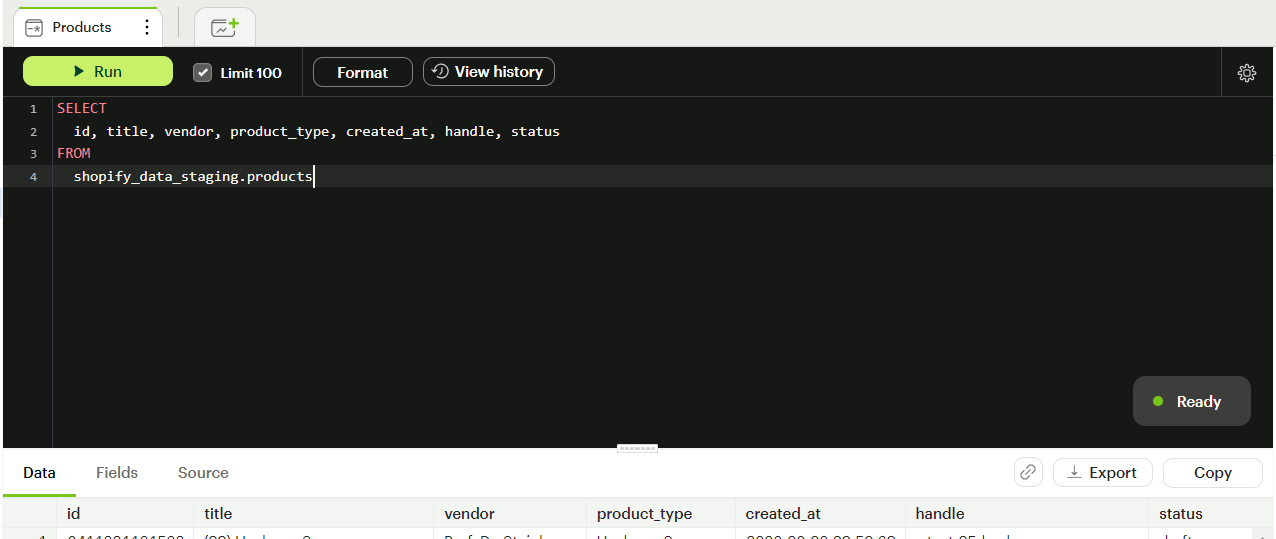
You can create a pipeline for the APIs discussed above by using dlt's REST API source. Let’s create a PokeAPI pipeline as an example. Follow these steps:

1. Create a Rest API source:

   dlt init rest_api duckdb
   

2. The following directory structure gets generated:

   rest_api_pipeline/
   ├── .dlt/
   │   ├── config.toml          # configs for your pipeline
   │   └── secrets.toml         # secrets for your pipeline
   ├── rest_api/                # folder with source-specific files
   │   └── ...
   ├── rest_api_pipeline.py     # your main pipeline script
   ├── requirements.txt         # dependencies for your pipeline
   └── .gitignore               # ignore files for git (not required)
   

3. Configure the source in rest_api_pipeline.py:

   def load_pokemon() -> None:
       pipeline = dlt.pipeline(
           pipeline_name="rest_api_pokemon",
           destination='duckdb',
           dataset_name="rest_api_data",
       )
   
       pokemon_source = rest_api_source(
           {
               "client": {
                   "base_url": "https://pokeapi.co/api/v2/",
               },
               "resource_defaults": {
                   "endpoint": {
                       "params": {
                           "limit": 1000,
                       },
                   },
               },
               "resources": [
                   "pokemon",
                   "berry",
                   "location",
               ],
           }
       )
   
   

For a detailed guide on creating a pipeline using the Rest API source, please read the Rest API source documentation here.

Example projects​

Here are some examples from dlt users and working students:

• A pipeline that pulls data from an API and produces a dashboard in the dbt blog.
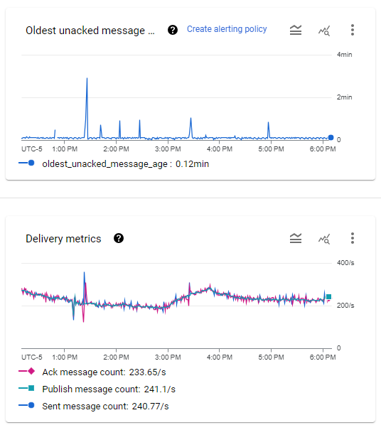
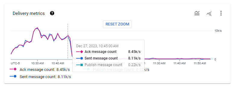
• A streaming pipeline on GCP that replaces expensive tools such as Segment/5tran with a setup 50-100x cheaper.
• Another streaming pipeline on AWS for a slightly different use case.
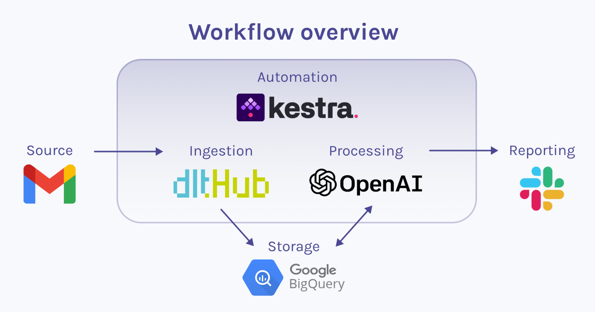
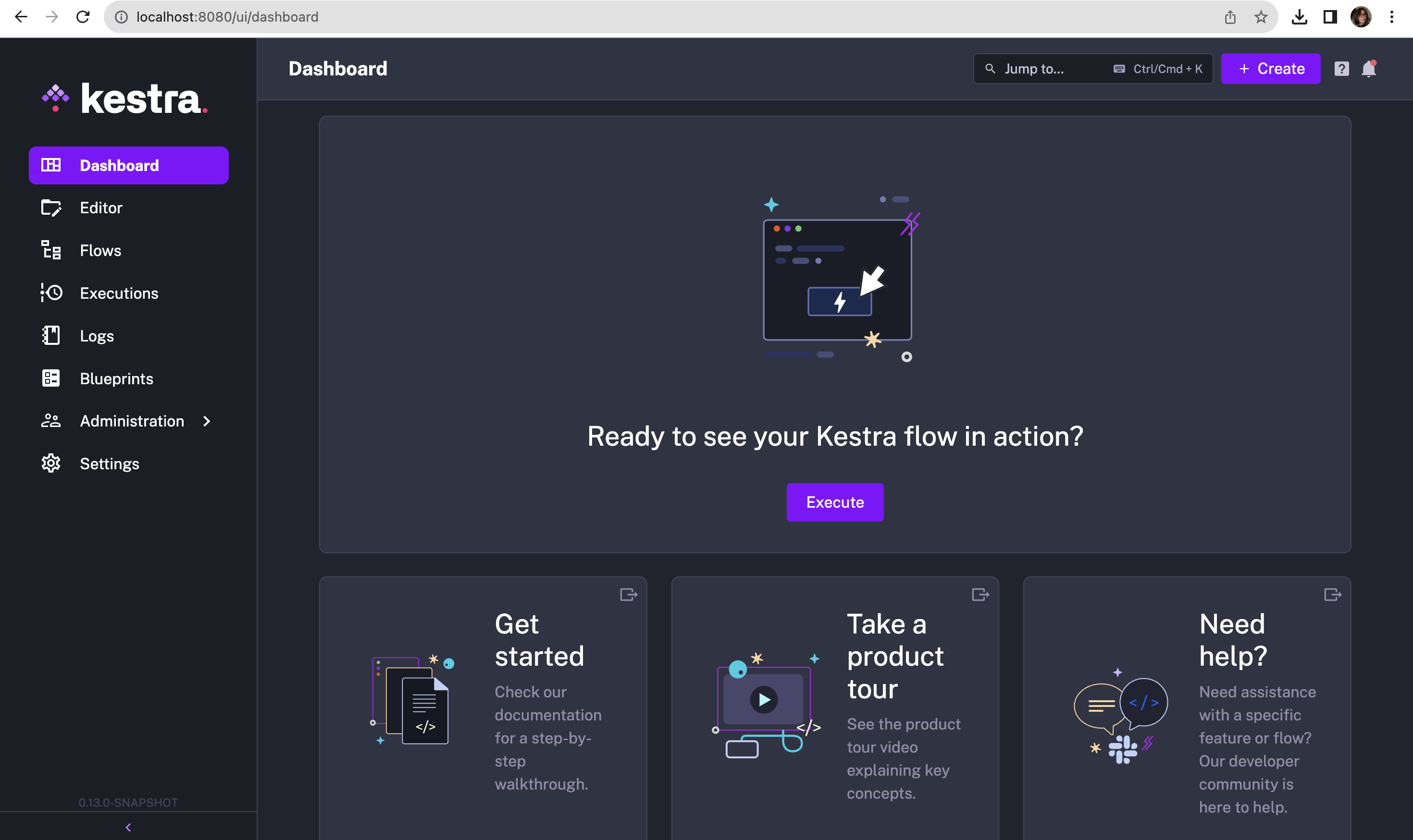
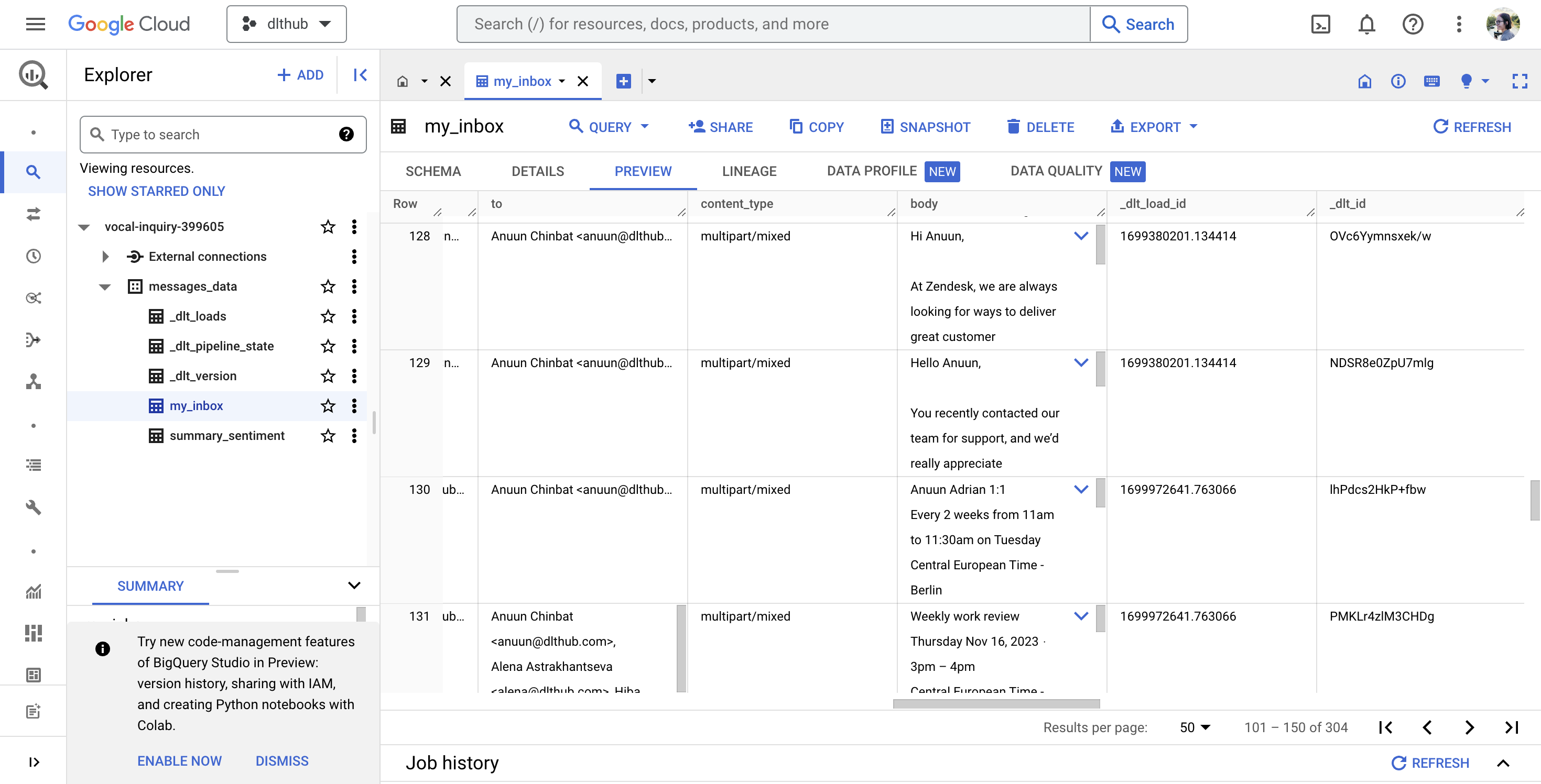
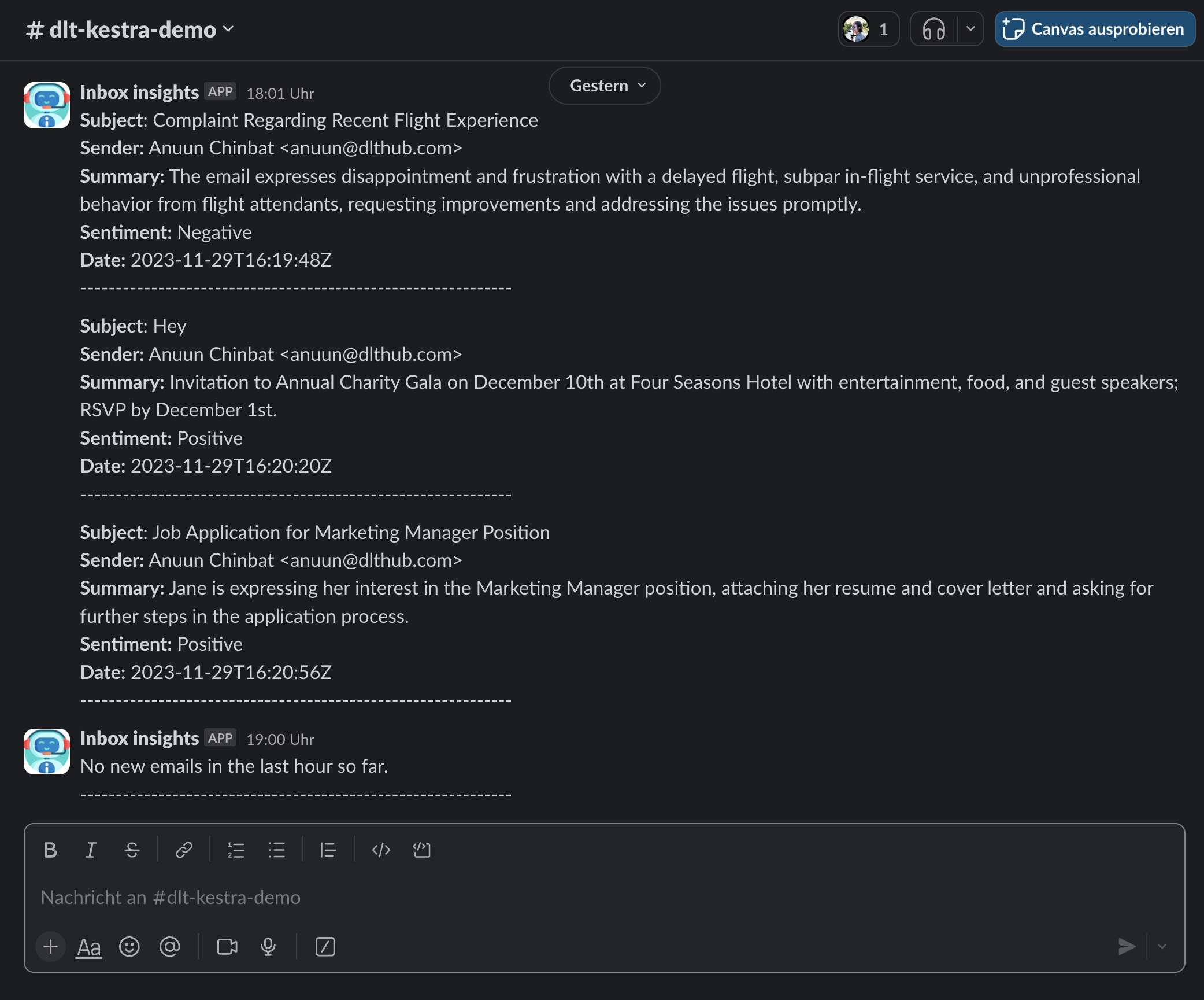
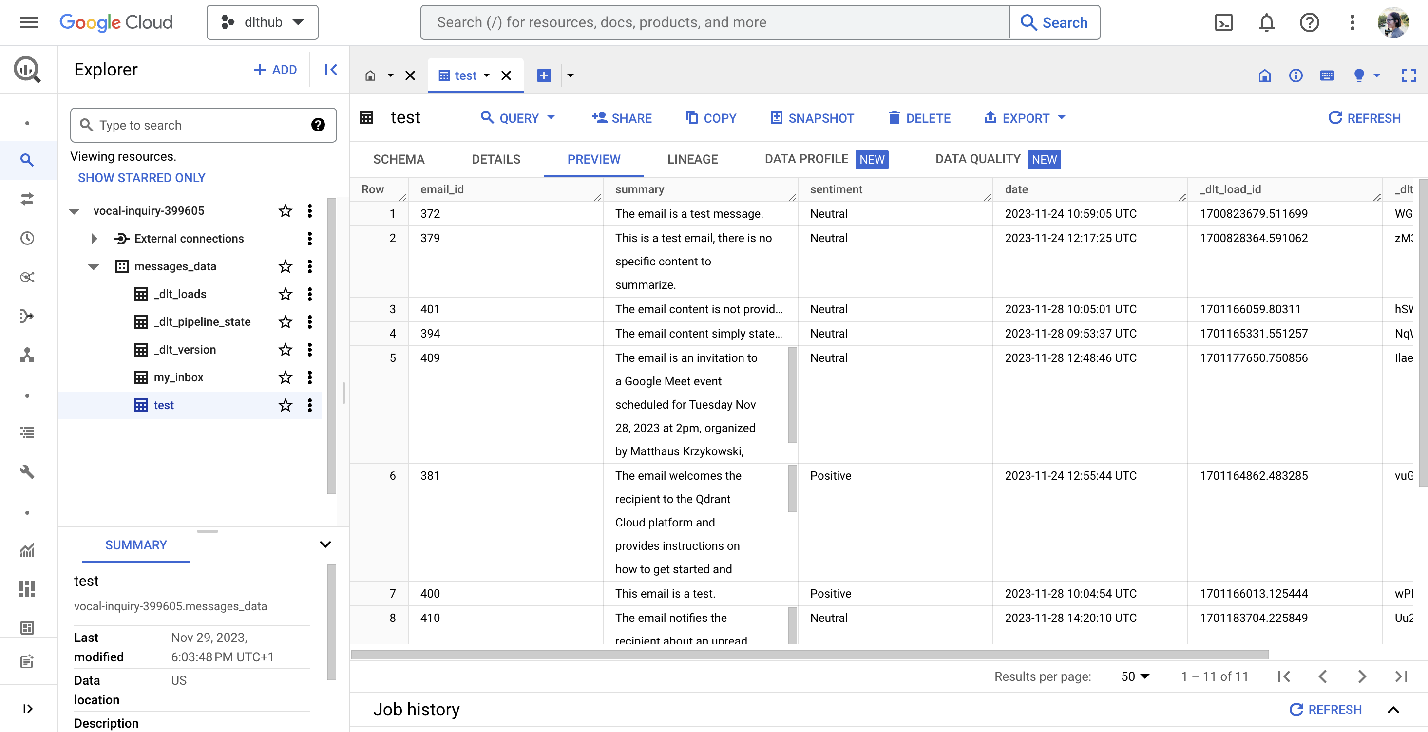
• Orchestrator + email + AI + Slack to summarize emails.
• Evaluate a frontend tool to show your ability to deliver end-to-end.
• An end-to-end data lineage implementation from extraction to dashboard.
• A bird pipeline and the associated schema management that ensures smooth operation Part 1, Part 2.
• Japanese language demos Notion calendar and exploring csv to bigquery with dlt.
• Demos with Dagster and Prefect.

DTC learners showcase​

Check out the incredible projects from our DTC learners:

1. e2e_de_project by scpkobayashi.
2. de-zoomcamp-project by theDataFixer.
3. data-engineering-zoomcamp2024-project2 by pavlokurochka.
4. de-zoomcamp-2024 by snehangsude.
5. zoomcamp-data-engineer-2024 by eokwukwe.
6. data-engineering-zoomcamp-alex by aaalexlit.
7. Zoomcamp2024 by alfredzou.
8. data-engineering-zoomcamp by el-grudge.

Explore these projects to see the innovative solutions and hard work the learners have put into their data engineering journeys!

Showcase your project​

If you want your project to be featured, let us know in the #sharing-and-contributing channel of our community Slack.

The Chinese Whisper of Data​

In the context of constructing a modern data stack through the development of various modular components for a data pipeline, our attention turns to the centralization of metrics and their definitions.

For the purposes of this demo, we’ll be looking specifically at how dlt and dbt come together to solve the problem of the data flow from data engineer → analytics engineer → data analyst → business user. That’s quite a journey. And just like any game of Chinese whisper, things certainly do get lost in translation.

To solve this problem, both these tools come together and seamlessly integrate to create everything from data sources to uniform metric definitions, that can be handled centrally, and hence are a big aid to the data democracy practices of your company!

Here’s how a pipeline could look:

1. Extract and load with dlt: dlt will automate data cleaning and normalization leaving you with clean data you can just use.
2. Create SQL models that simplify sources, if needed. This can include renaming and/or eliminating columns, identifying and setting down key constraints, fixing data types, etc.
3. Create and manage central metric definitions with the semantic layer.

1. Extract, Structure, & Load with dlt​

The data being used is of a questionnaire, which includes questions, the options of those questions, respondents and responses. This data is contained within a nested json object, that we’ll pass as a raw source to dlt to structure, normalize and dump into a BigQuery destination.

# initializing the dlt pipeline with your data warehouse destination
pipeline = dlt.pipeline(
    pipeline_name="survey_pipeline",
    destination="bigquery",
    dataset_name="questionnaire"
)

# running the pipeline (into a structured model)
# the dataset variable contains unstructured data
pipeline.run(dataset, table_name='survey')

The extract and load steps of an ETL pipeline have been taken care of with these steps. Here’s what the final structure looks like in BigQuery:

questionnaire is a well structured dataset with a base table, and child tables. The survey__questions and survey_questions__options are normalized tables with, the individual questions and options of those questions, respectively, connected by a foreign key. The same structure is followed with the ..__respondents tables, with survey__respondents__responses as our fact table.

2. Transformation with dbt​

For transformation, we head to dbt.

• The tables created by dlt are loaded as sources into dbt, with the same columns and structure as created by dlt.
• Since not much change is required to our original data, we can utilize the model creation ability of dbt to create a metric, whose results can directly be pulled by users.

Say, we would like to find the average age of people by their favorite color. First, we’d create an SQL model to find the age per person. The sources used are presented in the following image:

Next, using this information, we can find the average age for each favorite color. The sources used are as follows:

This is one method of centralizing a metric definition or formula, that you create a model out of it for people to directly pull into their reports.

3. Central Metric Definitions & Semantic Modelling with dbt​

The other method of creating a metric definition, powered by MetricFlow, is the dbt semantic layer. Using MetricFlow we define our metrics in yaml files and then directly query them from any different reporting tool. Hence, ensuring that no one gets a different result when they are trying to query company metrics and defining formulas and filters for themselves. For example, we created a semantic model named questionnaire, defining different entities, dimensions and measures. Like as follows:

model: ref('fact_table') # where the columns referred in this model will be taken from
# possible joining key columns
entities:
  - name: id
    type: primary
# where in SQL you would: create the aggregation column
measures:
  - name: surveys_total
    description: The total surveys for each --dimension.
    agg: count
    # if all rows need to be counted then expr = 1
    expr: 1
# where in SQL you would: group by columns
dimensions:
  # default dbt requirement
  - name: surveyed_at
    type: time
    type_params:
        time_granularity: day
  # count entry per answer
  - name: people_per_color
    type: categorical
    expr: answer
  # count entry per question
  - name: question
    type: categorical
    expr: question

Next, a metric is created from it:

metrics:
  - name: favorite_color
    description: Number of people with favorite colors.
    type: simple
    label: Favorite Colors
    type_params:
        # reference of the measure created in the semantic model
      measure: surveys_total
    filter: | # adding a filter on the "question" column for asking about favorite color
       {{  Dimension('id__question') }} = 'What is your favorite color?'

The DAG then looks like this:

We can now query this query, using whichever dimension we want. For example, here is a sample query: dbt sl query --metrics favorite_color --group-by id__people_per_color

The result of which is:

And just like that, the confusion of multiple people querying or pulling from different sources and different definitions get resolved. With aliases for different dimensions, the question of which column and table to pull from can be hidden - it adds a necessary level of abstraction for the average business end user.

dbt or “data build tool” has become a standard for transforming data in analytical environments. Most data pipelines nowadays start with ingestion and finish with running a dbt package.

dlt or “data load tool” is an open-source Python library for easily creating data ingestion pipelines. And of course, after ingesting the data, we want to transform it into an analytical model. For this reason, dlt offers a dbt runner that’s able to just run a dbt model on top of where dlt loaded the data, without setting up any additional things like dbt credentials.

Using dbt in Google Cloud functions​

To use dbt in cloud functions, we employed two methods:

1. dbt-core on GCP cloud functions.
2. dlt-dbt runner on GCP cloud functions.

Let’s discuss these methods one by one.

1. Deploying dbt-core on Google Cloud functions​

Let's dive into running dbt-core up on cloud functions.

You should use this option for scenarios where you have already collected and housed your data in a data warehouse, and you need further transformations or modeling of the data. This is a good option if you have used dbt before and want to leverage the power of dbt-core. If you are new to dbt, please refer to dbt documentation: Link Here.

Let’s start with setting up the following directory structure:

dbt_setup
|-- main.py
|-- requirements.txt
|-- profiles.yml
|-- dbt_project.yml
|-- dbt_transform
    |-- models
    |   |-- model1.sql
    |   |-- model2.sql
    |   |-- sources.yml
    |-- (other dbt related contents, if required)

You can setup the contents in dbt_transform folder by initing a new dbt project, for details refer to documentation.

To run dbt-core on GCP cloud functions:

1. Once you've tested the dbt-core package locally, update the profiles.yml before migrating the folder to the cloud function as follows:

   dbt_gcp: # project name
     target: dev # environment
     outputs:
       dev:
         type: bigquery
         method: oauth
         project: please_set_me_up! # your GCP project name
         dataset: please_set_me_up! # your project dataset name
         threads: 4
         impersonate_service_account: please_set_me_up! # GCP service account
   

   This service account should have bigquery read and write permissions.

2. Next, modify the main.py as follows:

   import os
   import subprocess
   import logging
   
   # Configure logging
   logging.basicConfig(level=logging.INFO)
   
   def run_dbt(request):
       try:
           # Set your dbt profiles directory (assuming it's in /workspace)
           os.environ['DBT_PROFILES_DIR'] = '/workspace/dbt_transform'
   
           # Log the current working directory and list files
           dbt_project_dir = '/workspace/dbt_transform'
           os.chdir(dbt_project_dir)
   
           # Log the current working directory and list files
           logging.info(f"Current working directory: {os.getcwd()}")
           logging.info(f"Files in the current directory: {os.listdir('.')}")
   
           # Run dbt command (e.g., dbt run)
   
           result = subprocess.run(
               ['dbt', 'run'],
               capture_output=True,
               text=True
               )
   
           # Return dbt output
           return result.stdout
   
       except Exception as e:
           logging.error(f"Error running dbt: {str(e)}")
           return f"Error running dbt: {str(e)}"
   

3. Next, list runtime-installable modules in requirements.txt:

   dbt-core
   dbt-bigquery
   

4. Finally, you can deploy the function using gcloud CLI as:

   gcloud functions deploy YOUR_FUNCTION_NAME \
   --gen2 \
   --region=YOUR_REGION \
   --runtime=python310 \
   --source=YOUR_SOURCE_LOCATION \
   --entry-point=YOUR_CODE_ENTRYPOINT \
   TRIGGER_FLAGS
   

   You have option to deploy the function via GCP Cloud Functions' GUI.

2. Deploying function using dlt-dbt runner​

The second option is running dbt using data load tool(dlt).

I work at dlthub and often create dlt pipelines. These often need dbt for modeling the data, making the dlt-dbt combination highly effective. For using this combination on cloud functions, we used dlt-dbt runner developed at dlthub.

The main reason I use this runner is because I load data with dlt and can re-use dlt’s connection to the warehouse to run my dbt package, saving me the time and code complexity I’d need to set up and run dbt standalone.

To integrate dlt and dbt in cloud functions, use the dlt-dbt runner; here’s how:

1. Lets start by creating the following directory structure:

   dbt_setup
   |-- main.py
   |-- requirements.txt
   |-- dbt_project.yml
   |-- dbt_transform
       |-- models
       |   |-- model1.sql
       |   |-- model2.sql
       |   |-- sources.yml
       |-- (other dbt related contents, if required)
   

   You can set up the dbt by initing a new project, for details refer to documentation.

   note

   With the dlt-dbt runner configuration, setting up a profiles.yml is unnecessary. DLT seamlessly shares credentials with dbt, and on Google Cloud Functions, it automatically retrieves service account credentials, if none are provided.

2. Next, configure the dbt_projects.yml and set the model directory, for example:

   model-paths: ["dbt_transform/models"]
   

3. Next, configure the main.py as follows:

   import dlt
   import logging
   from flask import jsonify
   from dlt.common.runtime.slack import send_slack_message
   from dlt.common import json
   
   def run_pipeline(request):
       """
       Set up and execute a data processing pipeline, returning its status
       and model information.
   
       This function initializes a dlt pipeline with pre-defined settings,
       runs the pipeline with a sample dataset, and then applies dbt
       transformations. It compiles and returns the information about
       each dbt model's execution.
   
       Args:
           request: The Flask request object. Not used in this function.
   
       Returns:
           Flask Response: A JSON response with the pipeline's status
           and dbt model information.
       """
       try:
           # Sample data to be processed
           data = [{"name": "Alice Smith", "id": 1, "country": "Germany"},
                   {"name": "Carlos Ruiz", "id": 2, "country": "Romania"},
                   {"name": "Sunita Gupta", "id": 3, "country": "India"}]
   
           # Initialize a dlt pipeline with specified settings
           pipeline = dlt.pipeline(
               pipeline_name="user_data_pipeline",
               destination="bigquery",
               dataset_name="dlt_dbt_test"
               )
   
           # Run the pipeline with the sample data
           pipeline.run(data, table_name="sample_data")
   
           # Apply dbt transformations and collect model information
           models = transform_data(pipeline)
           model_info = [
               {
                   "model_name": m.model_name,
                   "time": m.time,
                   "status": m.status,
                   "message": m.message
               }
               for m in models
           ]
   
           # Convert the model information to a string
           model_info_str = json.dumps(model_info)
   
           # Send the model information to Slack
           send_slack_message(
               pipeline.runtime_config.slack_incoming_hook,
               model_info_str
           )
   
           # Return a success response with model information
           return jsonify({"status": "success", "model_info": model_info})
       except Exception as e:
           # Log and return an error response in case of any exceptions
           logging.error(f"Error in running pipeline: {e}", exc_info=True)
   
           return jsonify({"status": "error", "error": str(e)}), 500
   
   def transform_data(pipeline):
       """
       Execute dbt models for data transformation within a dlt pipeline.
   
       This function packages and runs all dbt models associated with the
       pipeline, applying defined transformations to the data.
   
       Args:
           pipeline (dlt.Pipeline): The pipeline object for which dbt
           transformations are run.
   
       Returns:
           list: A list of dbt model run information, indicating the
           outcome of each model.
   
       Raises:
           Exception: If there is an error in running the dbt models.
       """
       try:
           # Initialize dbt with the given pipeline and virtual environment
           dbt = dlt.dbt.package(
               pipeline,
               "/workspace/dbt_transform",
               venv=dlt.dbt.get_venv(pipeline)
           )
           logging.info("Running dbt models...")
           # Run all dbt models and return their run information
           return dbt.run_all()
       except Exception as e:
           # Log and re-raise any errors encountered during dbt model
           # execution
           logging.error(f"Error in running dbt models: {e}", exc_info=True)
           raise
   
   # Main execution block
   if __name__ == "__main__":
       # Execute the pipeline function.
       run_pipeline(None)
   

4. The send_slack_message function is utilized for sending messages to Slack, triggered by both success and error events. For setup instructions, please refer to the official documentation here.

   RUNTIME__SLACK_INCOMING_HOOK was set up as environment variable in the above code.

5. Next, list runtime-installable modules in requirements.txt:

   dbt-core
   dbt-bigquery
   

6. Finally, you can deploy the function using gcloud CLI as:

   gcloud functions deploy YOUR_FUNCTION_NAME \
   --gen2 \
   --region=YOUR_REGION \
   --runtime=python310 \
   --source=YOUR_SOURCE_LOCATION \
   --entry-point=YOUR_CODE_ENTRYPOINT \
   TRIGGER_FLAGS
   

The merit of this method is that it can be used to load and transform data simultaneously. Using dlt for data loading and dbt for modeling makes using dlt-dbt a killer combination for data engineers and scientists, and my preferred choice. This method is especially effective for batched data and event-driven pipelines with small to medium workloads. For larger data loads nearing timeout limits, consider separating dlt and dbt into different cloud functions.

For more info on using dlt-dbt runner , please refer to the official documentation by clicking here.

Deployment considerations: How does cloud functions compare to Git Actions?​

At dlthub we already natively support deploying to GitHub Actions, enabling you to have a serverless setup with a 1-command deployment.

GitHub actions is an orchestrator that most would not find suitable for a data warehouse setup - but it certainly could do the job for a minimalistic setup. GitHub actions provide 2000 free minutes per month, so if our pipelines run for 66 minutes per day, we fit in the free tier. If our pipelines took another 1h per day, we would need to pay ~15 USD/month for the smallest machine (2 vCPUs) but you can see how that would be expensive if we wanted to run it continuously or had multiple pipelines always-on in parallel.

Cloud functions are serverless lightweight computing solutions that can handle small computational workloads and are cost-effective. dbt doesn't require the high computing power of the machine because it uses the computing power of the data warehouse to perform the transformations. This makes running dbt-core on cloud functions a good choice. The free tier would suffice for about 1.5h per day of running a 1 vCPU and 2 GB RAM machine, and if we wanted an additional 1h per day for this hardware it would cost us around 3-5 USD/month.

When deploying dbt-core on cloud functions, there are certain constraints to keep in mind. For instance, there is a 9-minute time-out limit for all 1st Gen functions. For 2nd Gen functions, there is a 9-minute limit for event-driven functions and a 60-minute limit for HTTP functions. Since dbt works on the processing power of the data warehouse it's operating on, 60 minutes is sufficient for most cases with small to medium workloads. However, it is important to remember the 9-minute cap when using event-driven functions.

Conclusion​

When creating lightweight pipelines, using the two tools together on one cloud function makes a lot of sense, simplifying the setup process and the handover between loading and transformation.

However, for more resource-intensive pipelines, we might want to improve resource utilisation by separating the dlt loading from the dbt running because while dbt’s run speed is determined by the database, dlt can utilize the cloud function’s hardware resources.

When it comes to setting up just a dbt package to run on cloud functions, I guess it comes to personal preference: I prefer dlt as it simplifies credential management. It automatically shares credentials with dbt, making setup easier. Streamlining the process further, dlt on Google Cloud functions, efficiently retrieves service account credentials, when none are provided. I also used dlt’s Slack error reporting function that sends success and error notifications from your runs directly to your Slack channel, helping me manage and monitor my runs.

Mode - Not another BI tool​

Empowering people by making data work simple - a value dlt embodies, and so does Mode. Both tools enable a person to build powerful things “on-the-fly”. Hence, when Mode positions itself as a self-service analytics platform, it delivers on that commitment by offering a user-friendly and familiar interface, and holistic experience.

👨🏻‍🦰, 👨🏻‍🦱, and 🧕🏻 from Logistics need to know what happened on the 1st of August, now!​

The sad story of most data and analytics teams are as follows: they are frequently burdened with routine (or ad-hoc) data requests, often involving simple SQL commands exported to Excel for external use. Despite the apparent simplicity, handling multiple requests simultaneously creates unnecessary workload. This detracts from the analytics team's capacity to engage in more constructive tasks such as cohort analysis, predictive analysis, hypothesis testing, creating funky plots - the fun stuff!

Nevertheless, employees outside the data team should not be blamed for making data requests without meaningful access to the data. If they were empowered to access and utilize the necessary data independently, individuals like 👨🏻‍🦰, 👨🏻‍🦱, and 🧕🏻 could filter user data from August 1st without relying on analysts.

Don’t know where you stand as a company, with data? Ask Mode​

You can start  your company’s journey with Mode by utilizing their data maturity test. It will tell you where you stand on your data democracy practices. A quick survey of user experiences showed exactly how Mode empowered companies of different sizes to become data thinkers. It has been adopted into 50% of Fortune 500 companies already!

Contrary to common belief, fostering a company-wide embrace of data thinking doesn't necessarily entail teaching everyone programming or conducting data science courses. Mode identifies four pivotal factors—people, processes, culture, and tools—that can empower companies to cultivate data thinkers. However, there are more reasons contributing to Mode's success in facilitating the emergence of company-wide "data heroes”. Let’s explore them.

The ease of adopting Mode​

👀 Familiarity & Simple UX​

Whether intentional or not, the table view on Mode, alongside by its green and white interface, evokes a sense of familiarity to original BI tool: Excel. Additionally, the platform offers the flexibility of having an SQL-only space and extending that functionality to incorporate Python (and R), providing a user experience similar to utilizing Databricks’ notebook & SQL environment. Lastly, the interface of the dashboarding spaces are the (simplified) experiences of tools like Power BI or Tableau.

When a tool feels familiar, people might embrace it faster. In Mode, all these familiar experiences are combined and simplified into one platform, and this holistic offering could be why Mode is: 1) easy to use and attracts users, and 2) easy to adopt across a company.

🔓 Access Paradigms​

Talking about company-wide adoption of a data tool, Mode offers various levels of access tailored to different user roles.

This aligns with the idea behind data democracy, ensuring that individuals throughout the company can engage with data. In Mode, this includes both viewing reports and deriving insights from them, and also viewing the underlying data collection (or datasets). Notably, access can be fine-tuned based on user distinctions, such as developers and business users. This is accomplished through nuanced permission settings and user grouping. By defining specific permissions, one can specify the actions users are empowered to perform. Now, let's explore the specific depth of what these users can actually do with all this power, in the next sections.

💽 SQL & Datasets​

Mode stores in itself “datasets”. This goes one step beyond writing a bajillion queries with joins and either saving them as code or saving them as materialized views in your database. You can use SQL and create datasets that are reusable and power a variety of different reports.

Contrast this with the user experience offered by other BI tools, even though they do offer the workspace for table creation, they lack robust documentation and centralization of these tables. It then becomes challenging for other teams (and in a couple of months, yourself) to comprehend the purpose and content of these tables - let alone use them across different reports.

There's no need to switch to a different database engine environment for SQL writing; Mode provides this functionality within its own environment. While tools like Databricks also offer this feature, Mode stands out by seamlessly utilizing it to generate shareable reports, much like the functionality seen in Metabase. Moreover, Mode goes a step further with its integration of Python and R, a capability present in Power BI but notably lacking the user-friendly interface of Mode's notebook environment.

🦉 A single source of truth!​

In creating these replicable datasets that can be accessed through different ways, Mode creates a single source of truth. This eliminates the need to search for disparate queries, streamlining the data retrieval (and access) process.

When we discuss data centralization, it typically involves cloud-hosted data warehouses that are accessible to authorized users at any time. This concept extends to business intelligence (BI) as well. Analysts within a company may utilize various tools, different source tables and SQL implementations, such as Apache Superset for business users, and Presto SQL for BI developers in their exploration, this leads to differences in loading and accessing data. Mode, in positioning itself as a central hub for data, resolves this by ensuring uniformity – everyone interacts with the same data source, eliminating variations in querying methods and results.

🔦 Semantic Layers (& dbt)​

Speaking of running around for different definitions, we come to the importance of the semantic layer in a data workflow.

In 2022, dbt introduced its semantic layer to address the challenge faced by BI developers and other stakeholders alike, in standardizing metric and indicator definitions across a company. This aimed to resolve issues arising from different individuals querying and defining these metrics, a process prone to human error (or logical code error) that can lead to inconsistencies. The significance of company-wide metrics lies in their impact on investors and their role in guiding teams on measuring growth and determining actions based on that growth.

Creating the Modern Data Stack with dlt & Mode​

Both dlt and Mode share the core value of data democracy, a cornerstone of the Modern Data Stack. When discussing the modern data stack, we are referring to the integration of various modular components that collaboratively create an accessible central system. Typically, this stack begins with a cloud data warehouse, where data is loaded, and updated by a data pipeline tool, like dlt. This process often involves a transformation layer, such as dbt, followed by the utilization of business intelligence (BI) tools like Mode.

In the context of a Python-based environment, one can employ dlt to ingest data into either a database or warehouse destination. Whether this Python environment is within Mode or external to it, dlt stands as its own independent data pipeline tool, responsible for managing the extract and load phases of the ETL process. Additionally, dlt has the ability to structure unstructured data within a few lines of code - this empowers individuals or developers to work independently.

With simplicity, centralization, and governance at its core, the combination of dlt and Mode, alongside a robust data warehouse, establishes two important elements within the modern data stack. Together, they handle data pipeline processes and analytics, contributing to a comprehensive and powerful modern data ecosystem.

There are two ways to use dlt and Mode to uncomplicate your workflows.

1. Extract, Normalize and Load with dlt and Visualize with Mode​

The data we are looking at comes from the source: Shopify. The configuration to initialize a Shopify source can be found in the dltHub docs. Once a dlt pipeline is initialized for Shopify, data from the source can be streamed into the destination of your choice. In this demo, we have chosen for it to be BigQuery destination. From where, it is connected to Mode. Mode’s SQL editor is where you can model your data for reports - removing all unnecessary columns or adding/subtracting the tables you want to be available to teams.

This stage can be perceived as Mode’s own data transformation layer, or semantic modelling layer, depending on which team/designation the user belongs to. Next, the reporting step is also simplified in Mode.

2. Use dlt from within the python workspace in Mode​

In this demo, we’ll forego the authentication issues of connecting to a data warehouse, and choose the DuckDB destination to show how the Python environment within Mode can be used to initialize a data pipeline and dump normalized data into a destination. In order to see how it works, we first install dlt[duckdb] into the Python environment.

!pip install dlt[duckdb]

Next, we initialize the dlt pipeline:

# initializing the dlt pipeline with your
# data warehouse destination
pipeline = dlt.pipeline(
        pipeline_name="mode_example_pipeline",
        destination="duckdb",
        dataset_name="staging_data")

And then, we pass our data into the pipeline, and check out the load information. Let's look at what the Mode cell outputs:

Let’s check if our pipeline exists within the Mode ecosystem:

Here we see the pipeline surely exists. Courtesy of Mode, anything that exists within the pipeline that we can query through Python can also be added to the final report or dashboard using the “Add to Report” button.

Once a pipeline is initialized within Mode’s Python environment, the Notebook cell can be frozen, and every consecutive run of the notebook can be a call to the data source, updating the data warehouse and reports altogether!

Conclusion​

dlt and Mode can be used together using either method, and make way for seamless data workflows. The first method mentioned in this article is the more traditional method of creating a data stack, where each tool serves a specific purpose. The second method, however utilizes the availability of a Python workspace within Mode to also serve the ETL process within Mode as well. This can be used for either ad-hoc reports and ad hoc data sources that need to be viewed visually, or, can be utilized as a proper pipeline creation and maintenance tool.

In the ever-evolving landscape of cloud computing, optimizing data workflows is paramount for achieving efficiency and scalability. Even though Google Cloud Platform offers the powerful Dataflow service to process data at scale, sometimes the simplest solution is worth a shot.

In cases with a relatively high Pub/Sub volume (>10 messages per second), a pull subscription with a continuously running worker is more cost-efficient and quicker than a push subscription. Using a combination of Docker, Instance Templates and Instance Groups, it is pretty simple to set up an auto-scaling group of instances that will process Pub/Sub messages.

This guide will walk you through the process of configuring GCP infrastructure that efficiently pulls JSON messages from a Pub/Sub subscription, infers schema, and inserts them directly into a Cloud SQL PostgreSQL database using micro-batch processing.

The issue at hand

In my current role at WishRoll, I was faced with the issue of processing a high amount of events and store them in the production database directly.

Imagine the scene: the server application produces analytics-style events such as "user logged-in", and "task X was completed" (among others). Eventually, for example, we want to run analytics queries on those events to count how many times a user logs in to better tailor their experience.

A. The trivial solution: synchronous insert​

The trivial solution is to synchronously insert these events directly in the database. A simple implementation would mean that each event fired results in a single insert to the database. This comes with 2 main drawbacks:

• Every API call that produces an event becomes slower. I.e. the /login endpoint needs to insert a record in the database
• The database is now hit with a very high amount of insert queries

With our most basic need of 2 event types, we were looking at about 200 to 500 events per second. I concluded this solution would not be scalable. To make it so, 2 things would be necessary: (1) make the event firing mechanism asynchronous and (2) bulk events together before insertion.

B. The serverless asynchronous solution​

A second solution is to use a Pub/Sub push subscription to trigger an HTTP endpoint when a message comes in. This would've been easy in my case because we already have a worker-style autoscaled App Engine service that could've hosted this. However, this only solves the 1st problem of the trivial solution; the events still come in one at a time to the HTTP service.

Although it's possible to implement some sort of bulking mechanism in a push endpoint, it's much easier to have a worker pull many messages at once instead.

C. The serverless, fully-managed Dataflow solution​

This led me to implement a complete streaming pipeline using GCP's streaming service: Dataflow. Spoiler: this was way overkill and led to weird bugs with DLT (data load tool). If you're curious, I've open-sourced that code too.

This solved both issues of the trivial solution, but proved pretty expensive and hard to debug and monitor.

D. An autoscaled asynchronous pull worker​

Disclaimer: I had never considered standalone machines from cloud providers (AWS EC2, GCP Compute Engine) to be a viable solution to my cloud problems. In my head, they seemed like outdated, manually provisioned services that could instead be replaced by managed services.

But here I was, with a need to have a continuously running worker. I decided to bite the bullet and try my luck with GCP Compute Engine. What I realized to my surprise, is that by using instance templates and instance groups, you can easily set up a cluster of workers that will autoscale.

The code is simple: run a loop forever that pulls messages from a Pub/Sub subscription, bulk the messages together, and then insert them in the database. Repeat.

Then deploy that code as an instance group that auto-scales based on the need to process messages.

Code walkthrough

The complete source code is available here.

Summarily, the code is comprised of 2 main parts:

• The pulling and batching logic to accumulate and group messages from Pub/Sub based on their destination table
• The load logic to infer the schema and bulk insert the records into the database. This part leverages DLT for destination compatibility and schema inference

Main loop​

By using this micro-batch architecture, we strive to maintain a balance of database insert efficiency (by writing multiple records at a time) with near real-time insertion (by keeping the window size around 5 seconds).

pipeline = dlt.pipeline(
    pipeline_name="pubsub_dlt",
    destination=DESTINATION_NAME,
    dataset_name=DATASET_NAME,
)

pull = StreamingPull(PUBSUB_INPUT_SUBCRIPTION)
pull.start()

try:
    while pull.is_running:
        bundle = pull.bundle(timeout=WINDOW_SIZE_SECS)
        if len(bundle):
            load_info = pipeline.run(bundle.dlt_source())
            bundle.ack_bundle()
            # pretty print the information on data that was loaded
            print(load_info)
        else:
            print(f"No messages received in the last {WINDOW_SIZE_SECS} seconds")

finally:
    pull.stop()

How to deploy​

The GitHub repo explains how to deploy the project as an instance group.

Database concerns​

Using DLT has the major advantage of inferring the schema of your JSON data automatically. This also comes with some caveats:

• The output schema of these analytics tables might change based on events
• If your events have a lot of possible properties, the resulting tables could become very wide (lots of columns) which is not something desirable in an OLTP database

Given these caveats, I make sure that all events fired by our app are fully typed and limited in scope. Moreover, using the table_name_data_key configuration of the code I wrote, it's possible to separate different events with different schemas into different tables.

See this README section for an example of application code and the resulting table.

Performance and cost

After running this code and doing backfills for a couple of weeks, I was able to benchmark the overall efficiency and cost of this solution.

Throughput capacity​

I am running a preemptible (SPOT) instance group of n1-standard-1 machines that auto-scales between 2 and 10 instances. In normal operation, a single worker can handle our load easily. However, because of the preemptible nature of the instances, I set the minimum number to 2 to avoid periods where no worker is running.

Maximum capacity​

When deploying the solution with a backlog of messages to process (15 hours worth of messages), 10 instances were spawned and cleared the backlog in about 25 minutes.

Between 7000 and 10000 messages per second were processed on average by these 10 instances, resulting in a minimum throughput capacity of 700 messages/s per worker.

Cost​

Using n1-standard-1 spot machines, this cluster costs $8.03/mth per active machine. With a minimum cluster size of 2, this means $16.06 per month.

Conclusion

Using more "primitive" GCP services around Compute Engine provides a straightforward and cost-effective way to process a high throughput of Pub/Sub messages from a pull subscription.

An important aspect of being a data person today is being able to navigate and choose from among many tools when setting up your company’s infrastructure. (And there are many tools out there!). While there is no one-size-fits-all when it comes to the right tooling, choosing ones that are powerful, flexible, and easily compatible with other tools empowers you to tailor your setup to your specific use case.

I am leading Data and Analytics at Taktile: a low-code platform used by global credit- and risk teams to design, build, and evaluate automated decision flows at scale. It’s the leading decision intelligence platform for the financial service industry today. To run our business effectively, we need an instrumentation mechanism that can anonymize and load millions of events and user actions each day into our Snowflake Data Warehouse. Inside the Warehouse, business users will use the data to run product analytics, build financial reports, set up automations, etc.

Choosing the right instrumentation engine is non-trivial​

Setting up the infrastructure to instrument a secured, high-volume data processing platform like Taktile is complicated and there are essential considerations that need to be made:

1. Data security: Each day, Taktile processes millions of high-stakes financial decisions for banks and Fintechs around the world. In such an environment, keeping sensitive data safe is crucial. Hence, Taktile only loads a subset of non-sensitive events into its warehouse and cannot rely on external vendors accessing decision data.
2. Handling irregular traffic volumes: Taktile’s platform is being used for both batch and real-time decision-making, which means that traffic spikes are common and hard to anticipate. Such irregular traffic mandates an instrumentation engine that can quickly scale out and guarantee timely event ingestion into the warehouse, even under high load.
3. Maintenance: a fast-growing company like Taktile needs to focus on its core product and on tools that don't create additional overhead.

dlt and AWS Lambda as the secure, scalable, and lightweight solution​

AWS Lambda is Amazon’s serverless compute service. dlt is a lightweight python ETL library that runs on any infrastructure. dlt fits neatly into the AWS Lambda paradigm, and by just adding a simple REST API and a few lines of python, it converts your Lambda function into a powerful and scalable event ingestion engine.

• Security: Lambda functions and dlt run within the perimeter of your own AWS infrastructure, hence there are no dependencies on external vendors.
• Scalability: serverless compute services like AWS Lambda are great at handling traffic volatility through built-in horizontal scaling.
• Maintenance: not only does AWS Lambda take care of provisioning and managing servers, but inserting dlt into the mix, also adds production-ready capabilities such as:
  • Automatic schema detection and evolution
  • Automatic normalization of unstructured data
  • Easy provisioning of staging destinations

Get started with dlt on AWS Lambda using SAM (AWS Serverless Application Model)​

SAM is a lightweight Infrastructure-As-Code framework provided by AWS. Using SAM, you simply declare serverless resources like Lambda functions, API Gateways, etc. in a template.yml file and deploy them to your AWS account with a lightweight CLI.

1. Install the SAM CLI [add link or command here]

   pip install aws-sam-cli
   

2. Define your resources in a template.yml file

   AWSTemplateFormatVersion: "2010-09-09"
   Transform: AWS::Serverless-2016-10-31
   
   Resources:
     ApiGateway:
       Type: AWS::Serverless::Api
       Properties:
         Name: DLT Api Gateway
         StageName: v1
     DltFunction:
       Type: AWS::Serverless::Function
       Properties:
         PackageType: Image
         Timeout: 30 # default is 3 seconds, which is usually too little
         MemorySize: 512 # default is 128mb, which is too little
         Events:
           HelloWorldApi:
             Type: Api
             Properties:
               RestApiId: !Ref ApiGateway
               Path: /collect
               Method: POST
         Environment:
           Variables:
             DLT_PROJECT_DIR: "/tmp" # the only writeable directory on a Lambda
             DLT_DATA_DIR: "/tmp" # the only writeable directory on a Lambda
             DLT_PIPELINE_DIR: "/tmp" # the only writeable directory on a Lambda
         Policies:
           - Statement:
               - Sid: AllowDLTSecretAccess
                 Effect: Allow
                 Action:
                   - secretsmanager:GetSecretValue
                 Resource: !Sub "arn:aws:secretsmanager:${AWS::Region}:${AWS::AccountId}:secret:DLT_*"
       Metadata:
         DockerTag: dlt-aws
         DockerContext: .
         Dockerfile: Dockerfile
   Outputs:
     ApiGateway:
       Description: "API Gateway endpoint URL for Staging stage for Hello World function"
       Value: !Sub "https://${ApiGateway}.execute-api.${AWS::Region}.amazonaws.com/v1/collect/"
   

3. Build a deployment package

   sam build
   

4. Test your setup locally

   sam local start-api
   
   # in a second terminal window
   curl -X POST http://127.0.0.1:3000/collect -d '{"hello":"world"}'
   

5. Deploy your resources to AWS

   sam deploy --stack-name=<your-stack-name> --resolve-image-repos --resolve-s3 --capabilities CAPABILITY_IAM
   

Caveats to be aware of when setting up dlt on AWS Lambda:​

No worries, all caveats described below are already being taken care of in the sample repo: https://github.com/codingcyclist/dlt-aws-lambda. I still recommend you read through them to be aware of what’s going on.

1. Local files: When running a pipeline, dlt usually stores a schema and other local files under your users’ home directory. On AWS Lambda, however, /tmp is the only directory into which files can be written. Simply tell dlt to use /tmp instead of the home directory by setting the DLT_PROJECT_DIR, DLT_DATA_DIR, DLT_PIPELINE_DIR environment variables to /tmp.
2. Database Secrets: dlt usually recommends providing database credentials via TOML files or environment variables. However, given that AWS Lambda does not support masking files or environment variables as secrets, I recommend you read database credentials from an external secret manager like AWS Secretsmanager (ASM).
3. Large dependencies: Usually, the code for a Lambda function gets uploaded as a .zip archive that cannot be larger than 250 MB in total (uncompressed). Given that dbt has a ~400 MB memory footprint (including Snowflake dependencies), the dlt Lambda function needs to be deployed as a Docker image, which can be up to 10 GB in size.

dlt and AWS Lambda are a great foundation for building a production-grade instrumentation engine​

dlt and AWS Lambda are a very powerful setup already. At Taktile, we still decided to add a few more components to our production setup to get even better resilience, scalability, and observability:

1. SQS message queue: An SQS message queue between the API gateway and the Lambda function is useful for three reasons. First, the queue serves as an additional buffer for sudden traffic spikes. Events can just fill the queue until the Lambda function picks them up and loads them into the destination. Second, an SQS queue comes with built-in batching so that the whole setup becomes even more cost-efficient. A batch of events only gets dispatched to the Lambda function when it reaches a certain size or has already been waiting in the queue for a specific period. Third, there is a dead-letter queue attached to make sure no events get dropped, even if the Lambda function fails. Failed events end up in the dead-letter queue and are sent back to the Lambda function once the root cause of the failure has been fixed.
2. Slack Notifications: Slack messages help a great deal in improving observability when running dlt in production. Taktile has set up Slack notifications for both schema changes and pipeline failures to always have transparency over the health status of their pipeline.

No matter whether you want to save time, cost, or both on your instrumentation setup, I hope you give dlt and AWS Lambda a try. It’s a modern, powerful, and lightweight combination of tools that has served us exceptionally well at Taktile.

THE PROBLEM​

There are two types of people: those who hoard thousands of unread emails in their inbox and those who open them immediately to avoid the ominous red notification. But one thing unites us all: everyone hates emails. The reasons are clear:

• They're often unnecessarily wordy, making them time-consuming.
• SPAM (obviously).
• They become black holes of lost communication because CC/BCC-ing people doesn't always work.
• Sometimes, there are just too many.

So, this post will explore a possible remedy to the whole email issue involving AI.

THE SOLUTION​

Don't worry; it's nothing overly complex, but it does involve some cool tools that everyone could benefit from.

💡 In a nutshell, I created two flows (a main flow and a subflow) in Kestra :

• The main flow extracts email data from Gmail and loads it into BigQuery using dlt, checks for new emails, and, if found, triggers the subflow for further processing.
• The subflow utilizes OpenAI to summarize and analyze the sentiment of an email, loads the results into BigQuery, and then notifies about the details via Slack.

Just so you're aware:

• Kestra is an open-source automation tool that makes both scheduled and event-driven workflows easy.
• dlt is an open-source library that you can add to your Python scripts to load data from various and often messy data sources into well-structured, live datasets.

HOW IT WORKS​

To lay it all out clearly: Everything's automated in Kestra, with hassle-free data loading thanks to dlt, and the analytical thinking handled by OpenAI. Here's a diagram to help you understand the general outline of the entire process.

Now, let's delve into specific parts of the implementation.

The environment:​

💡 The two flows in Kestra are set up in a very straightforward and intuitive manner. Simply follow the Prerequisites and Setup guidelines in the repo. It should take no more than 15 minutes.

Once you’ve opened http://localhost:8080/ in your browser, this is what you’ll see on your screen:

Now, all you need to do is create your flows and execute them.

The great thing about Kestra is its ease of use - it's UI-based, declarative, and language-agnostic. Unless you're using a task like a Python script, you don't even need to know how to code.

The data loading part​

💡 This is entirely managed by dlt in just five lines of code.

I set up a pipeline using the Inbox source – a regularly tested and verified source from dlt – with BigQuery as the destination.

In my scenario, the email data doesn't have nested structures, so there's no need for flattening. However, if you encounter nested structures in a different use case, dlt can automatically normalize them during loading.

Here's how the pipeline is defined and subsequently run in the first task of the main flow in Kestra:

# Run dlt pipeline to load email data from gmail to BigQuery
pipeline = dlt.pipeline(
    pipeline_name="standard_inbox",
    destination='bigquery',
    dataset_name="messages_data",
    dev_mode=False,
)

# Set table name
table_name = "my_inbox"
# Get messages resource from the source
messages = inbox_source(start_date = pendulum.datetime(2023, 11, 15)).messages
# Configure the messages resource to get bodies of the emails
messages = messages(include_body=True).with_name(table_name)
# Load data to the "my_inbox" table
load_info = pipeline.run(messages)

In this setup ☝️, dlt loads all email data into the table “my_inbox”, with the email body specifically stored in the “body” column. After executing your flow in Kestra, the table in BigQuery should appear as shown below:

The AI part​

💡 In this day and age, how can we not incorporate AI into everything? 😆

But seriously, if you're familiar with OpenAI, it's a matter of an API call to the chat completion endpoint. What simplifies it even further is Kestra’s OpenAI plugin.

In my subflow, I used it to obtain both the summary and sentiment analysis of each email body. Here's a glimpse of how it's implemented:

- id: get_summary
  type: io.kestra.plugin.openai.ChatCompletion
  apiKey: "{{ secret('OPENAI_API') }}"
  model: gpt-3.5-turbo
  prompt: "Summarize the email content in one sentence with less than 30 words: {{inputs.data[0]['body']}}"
  messages: [{"role": "system", "content": "You are a tool that summarizes emails."}]

The automation part​

💡 Kestra triggers are the ideal solution!

I’ve used a schedule trigger that allows you to execute your flow on a regular cadence e.g. using a CRON expression:

triggers:
  - id: schedule
    type: io.kestra.core.models.triggers.types.Schedule
    cron: "0 9-18 * * 1-5"

This configuration ensures that your flows are executed hourly on workdays from 9 AM to 6 PM.

THE OUTCOME​

A Slack assistant that delivers crisp inbox insights right at your fingertips:

And a well-organized table in BigQuery, ready for you to dive into a more complex analysis:

In essence, using Kestra and dlt offers a trio of advantages for refining email analysis and data workflows:

1. Efficient automation: Kestra effortlessly orchestrates intricate workflows, integrating smoothly with tools like dlt, OpenAI, and BigQuery. This process reduces manual intervention while eliminating errors, and freeing up more time for you.
2. User-friendly and versatile: Both Kestra and dlt are crafted for ease of use, accommodating a range of skill levels. Their adaptability extends to various use cases.
3. Seamless scaling: Kestra, powered by Kafka and Elasticsearch, adeptly manages large-scale data and complex workflows. Coupled with dlt's solid data integration capabilities, it ensures a stable and reliable solution for diverse requirements.

HOW IT COULD WORK ELSEWHERE​

Basically, you can apply the architecture discussed in this post whenever you need to automate a business process!

For detailed examples of how Kestra can be utilized in various business environments, you can explore Kestra's use cases.

Embrace automation, where the only limit is your imagination! 😛

In case you haven’t figured it out already, we at dltHub love creating blogs and demos. It’s fun, creative, and gives us a chance to play around with many new tools. We are able to do this mostly because, like any other modern tooling, dlt just fits in the modern ecosystem. Not only does dlt have existing integrations (to, for example, GCP, AWS, dbt, airflow etc.) that can simply be “plugged in”, but it is also very simple to customize it to integrate with almost any other modern tool (such as Metabase, Holistics, Dagster, Prefect etc.).

But what about enterprise systems like SAP? They are, after all, the most ubiquitous tooling out there: according to SAP data, 99 out of 100 largest companies are SAP customers. A huge part of the reason for this is that their ERP system is still the gold standard in terms of effectivity and reliability. However, when it comes to OLAP workloads like analytics, machine learning, predictive modelling etc., many companies prefer the convenience and cost savings of modern cloud solutions like GCP, AWS, Azure, etc..

So, wouldn’t it be nice to be able to integrate SAP into the modern ecosystem?

Unfortunately, this is not that simple. SAP does not integrate easily with non-SAP systems, and migrating data out from SAP is complicated and/or costly. This often means that ERP data stays separate from analytics data.

Creating a dlt integration​

Our users have been asking for SAP HANA data, hence I decided to create a custom dlt integration to SAP’s in-memory data warehouse: SAP HANA. Given its SQL backend and Python API, I figured dlt should also have no problem connecting to it.

I then use this pipeline to load SAP HANA tables into Snowflake, since Snowflake is cloud agnostic and can be run in different environments (such AWS, GCP, Azure, or any combination of the three). This is how I did it:

Step 1: I created an instance in SAP HANA cloud.

(I used this helpful tutorial to navigate SAP HANA.)

Step 2: I inserted some sample data.

Step 3: With tables created in SAP HANA, I was now ready to create a dlt pipeline to extract it into Snowflake:

Since SAP HANA has a SQL backend, I decided to extract the data using dlt’s SQL source

1. I first created a dlt pipeline

   dlt init sql_database snowflake

2. I then passed the connection string for my HANA instance inside the loading function in sql_database_pipeline.py. (Optional: I also specified the tables that I wanted to load in sql_database().with_resources("v_city", "v_hotel", "room") )

3. Before running the pipeline I installed all necessary requirements using

   pip install -r requirements.txt

   The dependencies inside requirements.txt are for the general SQL source. To extract data specifically from HANA, I also installed the packages hdbcli and sqlalchemy-hana.

Step 4: I finally ran the pipeline using python sql_database_pipeline.py. This loaded the tables into Snowflake.

Takeaway​

The dlt SAP HANA connector constructed in this demo works like any other dlt connector, and is able to successfully load data from SAP HANA into data warehouses like Snowflake.

Furthermore, the demo only used a toy example, but the SQL source is a production-ready source with incremental loading, merges, data contracts etc., which means that this pipeline could also be configured for production use-cases.

Finally, the dlt-SAP integration has bigger consequences: it allows you to add other tools like dbt, airflow etc. easily into an SAP workflow, since all of these tools integrate well with dlt.

Next steps​

This was a just first step into exploring what’s possible. Creating a custom dlt connector worked pretty well for SAP HANA, and there are several possible next steps, such as converting this to a verified source, or building other SAP connectors.

1. Creating a verified source for SAP HANA: This should be pretty straight-forward since it would require a small modification of the existing SQL source.
2. Creating a dlt connector for SAP S/4 HANA: S/4 HANA is SAP’s ERP software that runs on the HANA database. The use case would be to load ERP tables from S/4 HANA into other data warehouses like Snowflake. Depending on the requirements, there are two ways to go about it:
   1. Low volume data: This would again be straight-forward. SAP offers REST API end points to access ERP tables, and dlt is designed to be able to load data from any such end point.
   2. High volume data: dlt can also be configured for the use case of migrating large volumes of data with fast incremental or merge syncs. But this would require some additional steps, such as configuring the pipeline to access HANA backend directly from Python hdbcli.

Why data lineage is important?​

Data lineage is an important tool in an arsenal of a data engineer. It showcases the journey of data from its source to its destination. It captures all the pitstops made and can help identify issues in the data pipelines by offering a birds eye view of the data.

As data engineers, data lineage enables us to trace and troubleshoot the datapoints we offer to our stakeholders. It is also an important tool that can be used to meet regulation regarding privacy. Moreover, it can help us evaluate how any changes upstream in a pipeline effects the downstream source. There are many types of data lineage, the most commonly used types are the following:

• Table lineage, it shows the raw data sources that are used to form a new table. It tracks the flow of data, showing how data moves forward through various processes and transformations.
• Row lineage reveals the data flow at a more granular level. It refers to tracking and understanding of individual rows of data as they move through various stages in a data processing pipeline. It is a subset of table lineage that focuses specifically on the journey of individual records or rows rather than the entire dataset.
• Column lineage specifically focuses on tracking and documenting the flow and transformation of individual columns or fields within different tables and views in the data.

Project Overview​

In this demo, we showcase how you can leverage the dlt pipeline load_info to create table, row and column lineage for your data. The code for the demo is available on GitHub.

The dlt load_info encapsulates useful information pertaining the loaded data. It contains the pipeline, dataset name, the destination information and list of loaded packages among other elements. Within the load_info packages, you will find a list of all tables and columns created at the destination during loading of the data. It can be used to display all the schema changes that occur during data ingestion and implement data lineage.

We will work with the example of a skate shop that runs an online shop using Shopify, in addition to its physical stores. The data from both sources is extracted using dlt and loaded into BigQuery.

In order to run analytics workloads, we will create a transformed fact_sales table using dbt and the extracted raw data. The fact_sales table can be used to answer all the sales related queries for the business.

The load_info produced by dlt for both pipelines is also populated into BigQuery. We will use this information to create a Dashboard in Metabase that shows the data lineage for the fact_sales table.

Implementing Data Lineage​

To get started install dlt and dbt:

pip install dlt
pip install dbt-bigquery

As we will be ingesting data into BigQuery, we first need to create service account credentials for BigQuery. You can find more info on setting up a service account in the dlt docs.

We use the following CSV files as our data sources for this demo:

• Test Shopify data
• Kaggle Supermarket dataset.

dlt provides verified Shopify source to directly extract data from the Shopify API.

Step 1: Initialize a dlt pipeline​

To get started we initialize a dlt pipeline and selecting BigQuery as our destination by running the following command:

dlt init data_lineage bigquery

This will create default scaffolding to build our pipeline. Install the dependencies by running the following command:

pip install -r requirements.txt

Loading the data​

As a first step, we will load the sales data from the online and physical store of the skate shop into BigQuery. In addition to the sales data, we will also ingest the dlt load_info into BigQuery. This will help us track changes in our pipeline.

Step 2: Adding the dlt pipeline code​

In the data_lineage.py file remove the default code and add the following:

FILEPATH = "data/supermarket_sales.csv"
FILEPATH_SHOPIFY = "data/orders_export_1.csv"

class Data_Pipeline:
    def __init__(self, pipeline_name, destination, dataset_name):
        self.pipeline_name = pipeline_name
        self.destination = destination
        self.dataset_name = dataset_name

    def run_pipeline(self, data, table_name, write_disposition):
        # Configure the pipeline with your destination details
        pipeline = dlt.pipeline(
            pipeline_name=self.pipeline_name,
            destination=self.destination,
            dataset_name=self.dataset_name
        )
        # Run the pipeline with the provided data
        load_info = pipeline.run(
            data,
            table_name=table_name,
            write_disposition=write_disposition
        )

        # Pretty print the information on data that was loaded
        print(load_info)
        return load_info

Any changes in the underlying data are captured by the dlt load_info. To showcase this, we will filter the data to remove the Branch and Tags columns from Store and Shopify data respectively and run the pipeline. Later we will add back the columns and rerun the pipeline. These new columns added will be recorded in the load_info packages.

We will add the load_info back to BigQuery to use in our Dashboard. The Dashboard will provide an overview data lineage for our ingested data.

if __name__ == "__main__":

    data_store = pd.read_csv(FILEPATH)
    data_shopify = pd.read_csv(FILEPATH_SHOPIFY)

    #filtering some data.
    select_c_data_store = data_store.loc[
        :, data_store.columns.difference(['Branch'])
    ]
    select_c_data_shopify = data_shopify.loc[
        :, data_shopify.columns.difference(['Tags'])
    ]

    pipeline_store = Data_Pipeline(
        pipeline_name='pipeline_store',
        destination='bigquery',
        dataset_name='sales_store'
    )
    pipeline_shopify = Data_Pipeline(
        pipeline_name='pipeline_shopify',
        destination='bigquery',
        dataset_name='sales_shopify'
    )

    load_a = pipeline_store.run_pipeline(
        data=select_c_data_store,
        table_name='sales_info',
        write_disposition='replace'
    )
    load_b = pipeline_shopify.run_pipeline(
        data=select_c_data_shopify,
        table_name='sales_info',
        write_disposition='replace'
    )

    pipeline_store.run_pipeline(
        data=load_a.load_packages,
        table_name="load_info",
        write_disposition="append"
    )
    pipeline_shopify.run_pipeline(
        data=load_b.load_packages,
        table_name='load_info',
        write_disposition="append"
    )

Step 3: Run the dlt pipeline​

To run the pipeline, execute the following command:

python data_lineage.py

This will load the data into BigQuery. We now need to remove the column filters from the code and rerun the pipeline. This will add the filtered columns to the tables in BigQuery. The change will be captured by dlt.

Data Transformation and Lineage​

Now that both the Shopify and Store data are available in BigQuery, we will use dbt to transform the data.

Step 4: Initialize a dbt project and define model​

To get started initialize a dbt project in the root directory:

dbt init sales_dbt

Next, in the sales_dbt/models we define the dbt models. The first model will be the fact_sales.sql. The skate shop has two data sources: the online Shopify source and the physical Store source. We need to combine the data from both sources to create a unified reporting feed. The fact_sales table will be our unified source.

Code for fact_sales.sql:

{{ config(materialized='table') }}

select
  invoice_id,
  city,
  unit_price,
  quantity,
  total,
  date,
  payment,
  info._dlt_id,
  info._dlt_load_id,
  loads.schema_name,
  loads.inserted_at
from {{source('store', 'sales_info')}} as info
left join {{source('store', '_dlt_loads')}} as loads
on  info._dlt_load_id = loads.load_id

union all

select
  name as invoice_id,
  billing_city,
  lineitem_price,
  lineitem_quantity,
  total,
  created_at,
  payment_method,
  info._dlt_id,
  info._dlt_load_id,
  loads.schema_name,
  loads.inserted_at
from {{source('shopify', 'sales_info')}} as info
left join {{source('shopify', '_dlt_loads')}} as loads
on  info._dlt_load_id = loads.load_id
where financial_status = 'paid'

In the query, we join the sales information for each source with its dlt load_info. This will help us keep track of the number of rows added with each pipeline run. The schema_name identifies the source that populated the table and helps establish the table lineage. While the _dlt_load_id identifies the pipeline run that populated the each row and helps establish row level lineage. The sources are combined to create a fact_sales table by doing a union over both sources.

Next, we define the schema_change.sql model to capture the changes in the table schema using a following query:

{{ config(materialized='table') }}

select *
from {{source('store', 'load_info__tables__columns')}}

union all

select *
from {{source('shopify', 'load_info__tables__columns')}}

In the query, we combine the load_info for both sources by doing a union over the sources. The resulting schema_change table contains records of the column changes that occur on each pipeline run. This will help us track the column lineage and will be used to create our Data Lineage Dashboard.

Step 5: Run the dbt package​

In the data_lineage.py add the code to run the dbt package using dlt.

pipeline_transform = dlt.pipeline(
    pipeline_name='pipeline_transform',
    destination='bigquery',
    dataset_name='sales_transform'
)

venv = Venv.restore_current()
here = os.path.dirname(os.path.realpath(__file__))

dbt = dlt.dbt.package(
    pipeline_transform,
    os.path.join(here, "sales_dbt/"),
    venv=venv
)

models = dbt.run_all()

for m in models:
    print(
        f"Model {m.model_name} materialized in {m.time} - "
        f"Status {m.status} and message {m.message}"
    )

Next, run the pipeline using the following command:

python data_lineage.py

Once the pipeline is run, a new dataset called sales_transform will be created in BigQuery, which will contain the fact_sales and schema_changes tables that we defined in the dbt package.

Step 6: Visualising the lineage in Metabase​

To access the BigQuery data in Metabase, we need to connect BigQuery to Metabase. Follow the Metabase docs to connect BigQuery to Metabase.

Once BigQuery is connected with Metabase, use the SQL Editor to create the first table. The Data Load Overview table gives an overview of the dlt pipelines that populated the fact_sales table. It shows the pipeline names and the number of rows loaded into the fact_sales table by each pipeline.

This can be used to track the rows loaded by each pipeline. An upper and lower threshold can be set, and when our pipelines add rows above or below the threshold, that can act as our canary in the coal mine.

Next, we will visualize the fact_sales and the schema_changes as a table and add the dlt_load_id as a filter. The resulting Data Lineage Dashboard will give us an overview of the table, row and column level lineage for our data.

When we filter by the dlt_load_id the dashboard will filter for the specific pipeline run. In the Fact Sales table the column schema_name identifies the raw sources that populated the table (Table lineage). The table also shows only the rows that were added for the pipeline run (Row Lineage). Lastly, the Updated Columns table revels the columns that were added for filtered pipeline run (Column Lineage).

When we ran the pipeline initially, we filtered out the Tags column and later reintroduced it and ran the pipeline again. The Updated Columns shows that the Tags column was added to the Fact Sales table with the new pipeline run.

Conclusion​

Data lineage provides an overview of the data journey from the source to destination. It is an important tool that can help troubleshoot a pipeline. dlt load_info provides an alternative solution to visualizing data lineage by tracking changes in the underlying data.

Although dlt currently does not support data flow diagrams, it tracks changes in the data schema that can be used to create dashboards that provides an overview of table, row and column lineage for the loaded data.

💡 This article explores methods for monitoring transactional events, allowing immediate action and data capture that might be lost otherwise. We focus on Github, Slack, and Hubspot, demonstrating techniques applicable to low-volume transactional events (under 500k/month) within the free tier. For clickstream tracking or higher volumes, we recommend more scalable solutions.

There’s more than one way to sync data. Pulling data after it has been collected from APIs is a classic way, but some types of data are better transmitted as an event at the time of happening. Our approach is event-triggered and can include actions like:

These actions initiate a webhook that sends a POST request to trigger a DLT pipeline for event ingestion. The data is then loaded into BigQuery.

This setup enables real-time alerts or event storage for later use. For example, let’s say you want to alert every time something happens - you’d want to be able to capture an event being sent to you and act on it. Or, in some cases, you store it for later use. This guide covers a use case for deploying and setting up webhooks.

Why do we use webhooks?​

Whenever we want to receive an event from an external source, we need a “recipient address” to which they can send the data. To solve this problem, an effortless way is to use a URL as the address and accept a payload as data.

Why cloud functions?​

The key reasons for using cloud functions include:

1. To have a URL up and accept the data payload, we would need some service or API always to be up and ready to listen for the data.

2. Creating our application for this would be cumbersome and expensive. It makes sense to use some serverless service for low volumes of events.

3. On AWS, you would use API gateway + lambda to handle incoming events, but for GCP users, the option is more straightforward: Google Cloud functions come with an HTTP trigger, which enables you to create a URL and accept a payload.

4. The pricing for cloud functions is unbeatable for low volumes: For ingesting an event with a minor function, assuming processing time to be a few seconds, we could invoke a few hundred thousand calls every month for free. For more pricing details, see the GCP pricing page for cloud functions.

Let's dive into the deployment of webhooks and app setup, focusing next on triggers from GitHub, Slack, and HubSpot for use cases discussed above.

1. GitHub Webhook​

This GitHub webhook is triggered upon specified events such as pull requests (PRs), commits, or comments. It relays relevant data to BigQuery. Set up the GitHub webhook by creating the cloud function URL and configuring it in the GitHub repository settings.

1.1 Initialize GitHub webhook deployment​

To set up the webhook, start by creating a cloud function. Follow these brief steps, and for an in-depth guide, please refer to the detailed documentation.

1. Log into GCP and activate the Cloud Functions API.

2. Click 'Create Function' in Cloud Functions, and select your region and environment setup.

3. Choose HTTP as the trigger, enable 'Allow unauthenticated invocations', save, and click 'Next'.

4. Set the environment to Python 3.10 and prepare to insert code into main.py:

   import dlt
   import time
   from google.cloud import bigquery
   from dlt.common import json
   
   def github_webhook(request):
       # Extract relevant data from the request payload
       data = request.get_json()
   
       Event = [data]
   
       pipeline = dlt.pipeline(
           pipeline_name='platform_to_bigquery',
           destination='bigquery',
           dataset_name='github_data',
       )
   
       pipeline.run(Event, table_name='webhook') #table_name can be customized
       return 'Event received and processed successfully.'
   

5. Name the function entry point "github_webhook" and list required modules in requirements.txt.

   # requirements.txt
   dlt[bigquery]
   

6. Post-deployment, a webhook URL is generated, typically following a specific format.

   https://{region]-{project-id}.cloudfunctions.net/{cloud-function-name}
   

Once the cloud function is configured, it provides a URL for GitHub webhooks to send POST requests, funneling data directly into BigQuery.

1.2 Configure the repository webhook in GitHub​

Set up a GitHub repository webhook to trigger the cloud function on specified events by following these steps:

1. Log into GitHub and go to your repository.
2. Click "Settings" > "Webhooks" > "Add webhook."
3. Enter the cloud function URL in "Payload URL."
4. Choose "Content-Type" and select events to trigger the webhook, or select "Just send me everything."
5. Click "Add webhook."

With these steps complete, any chosen events in the repository will push data to BigQuery, ready for analysis.

2. Slack Webhook​

This Slack webhook fires when a user sends a message in a channel where the Slack app is installed. To set it up, set up a cloud function as below and obtain the URL, then configure the message events in Slack App settings.

2.1 Initialize Slack webhook deployment​

Set up the webhook by creating a cloud function, using the same steps as for the GitHub webhook.

1. Here’s what main.py looks like:

   import dlt
   from flask import jsonify
   
   def slack_webhook(request):
       # Handles webhook POST requests
       if request.method == 'POST':
           data = request.get_json()
   
           # Responds to Slack's verification challenge
           if 'challenge' in data:
               return jsonify({'challenge': data['challenge']})
   
           # Processes a message event
           if 'event' in data and 'channel' in data['event']:
               message_data = process_webhook_event(data['event'])
   
               # Configures and initiates a DLT pipeline
               pipeline = dlt.pipeline(
                   pipeline_name='platform_to_bigquery',
                   destination='bigquery',
                   dataset_name='slack_data',
               )
   
               # Runs the pipeline with the processed event data
               pipeline.run([message_data], table_name='webhook')
               return 'Event processed.'
           else:
               return 'Event type not supported', 400
       else:
           return 'Only POST requests are accepted', 405
   
   def process_webhook_event(event_data):
       # Formats the event data for the DLT pipeline
       message_data = {
           'channel': event_data.get('channel'),
           'user': event_data.get('user'),
           'text': event_data.get('text'),
           'ts': event_data.get('ts'),
           # Potentially add more fields according to event_data structure
       }
       return message_data
   

2. Name the entry point "slack_webhook" and include the necessary modules in requirements.txt, the same as the GitHub webhook setup.

3. Once the cloud function is configured, you get a URL for Slack events to send POST requests, funneling data directly into BigQuery.

2.2 Set up and configure a Slack app​

Create and install a Slack app in your workspace to link channel messages from Slack to BigQuery as follows:

1. Go to "Manage apps" in workspace settings; click "Build" and "Create New App".
2. Choose "from scratch", name the app, select the workspace, and create the app.
3. Under "Features", select "Event Subscription", enable it, and input the Cloud Function URL.
4. Add message.channels under "Subscribe to bot events".
5. Save and integrate the app to the desired channel.

With these steps complete, any message sent on the channel will push data to BigQuery, ready for analysis.

3. Hubspot webhook​

A Hubspot webhook can be configured within an automation workflow, applicable to contacts, companies, deals, tickets, quotes, conversations, feedback submissions, goals and invoices. It triggers upon specific conditions or data filters. To establish it, create a cloud function, retrieve its URL, and input this in Hubspot's automation workflow settings for message events.

3.1 Initialize Hubspot webhook deployment​

Set up the webhook by creating a cloud function, using the same steps as for the GitHub webhook.

1. Here’s what main.pylooks like:

   import dlt
   from flask import jsonify
   
   def hubspot_webhook(request):
       # Endpoint for handling webhook POST requests from Hubspot
       if request.method == 'POST':
           # Get JSON data from the POST request
           data = request.get_json()
   
           # Initialize and configure the DLT pipeline
           pipeline = dlt.pipeline(
               pipeline_name="hubspot",
               destination='bigquery',               # Destination service for the data
               dataset_name='hubspot_webhooks_dataset',  # BigQuery dataset name
           )
   
           # Execute the pipeline with the incoming data
           pipeline.run([data], table_name='hubspot_contact_events')
   
           # Return a success response
           return jsonify(message='HubSpot event processed.'), 200
       else:
           # Return an error response for non-POST requests
           return jsonify(error='Only POST requests are accepted'), 405
   
   

2. Name the entry point "your_webhook" and include the necessary modules in requirements.txt, the same as the GitHub webhook setup.

3. Once the cloud function is configured, you get a URL for Slack events to send POST requests, funneling data directly into BigQuery.

3.2 Configure a Hubspot automation workflow​

To activate a Hubspot workflow with your webhook:

1. Go to Hubspot: "Automation" > "Workflows" > "Create workflow".
2. Start from scratch; choose "Company-based" for this example.
3. Set "Object created" as the trigger.
4. Add the "Send a webhook" action, use the "POST" method, and input your webhook URL.
5. Select the company properties to include, test, and save.

This triggers the webhook upon new company creation, sending data to Bigquery via DLT.

In conclusion​

Setting up a webhook is straightforward.

Using dlt with schema evolution, we can accept the events without worrying about their schema. However, for events with custom schemas or vulnerable to bad data quality or abuse, consider using dlt’s data contracts.